Kepler Power Attribution Guide

This guide explains how Kepler measures and attributes power consumption to processes, containers, VMs, and pods running on a system.

Bird's Eye View

The Big Picture

Modern systems lack per-workload energy metering, providing only aggregate power consumption at the hardware level. Kepler addresses this attribution challenge through proportional distribution based on resource utilization:

Hardware Energy Collection - Intel RAPL sensors provide cumulative energy counters at package, core, DRAM, and uncore levels
System Activity Analysis - CPU utilization metrics from /proc/stat determine the ratio of active vs idle system operation
Power Domain Separation - Total energy is split into active power (proportional to workload activity) and idle power (baseline consumption)
Proportional Attribution - Active power is distributed to workloads based on their CPU time consumption ratios

Core Philosophy

Kepler implements a CPU-time-proportional energy attribution model that distributes hardware-measured energy consumption to individual workloads based on their computational resource usage patterns.

The fundamental principle recognizes that system power consumption has two distinct components:

Active Power: Energy consumed by computational work, proportional to CPU utilization and scalable with workload activity
Idle Power: Fixed baseline energy for maintaining system operation, including memory refresh, clock distribution, and idle core power states

Attribution Formula

All workload types use the same proportional attribution formula:

Workload Power = (Workload CPU Time Δ / Node CPU Time Δ) × Active Power

This ensures energy conservation - the sum of attributed power remains proportional to measured hardware consumption while maintaining fairness based on actual resource utilization.

Power Attribution Diagram

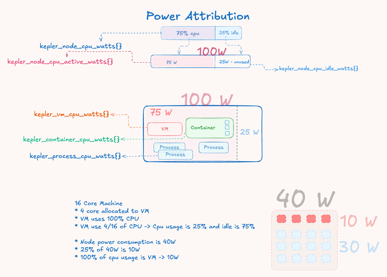
Figure 1: Power attribution flow showing how total measured power is decomposed into active and idle components, with active power distributed proportionally based on workload CPU time deltas.

Multi-Socket and Zone Aggregation

Modern server systems often feature multiple CPU sockets, each with their own RAPL energy domains. Kepler handles this complexity through zone aggregation:

Zone Types and Hierarchy:

Package zones: CPU socket-level energy (e.g., package-0, package-1)
Core zones: Individual CPU core energy within each package
DRAM zones: Memory controller energy per socket
Uncore zones: Integrated GPU, cache, and interconnect energy
PSys zones: Platform-level energy (most comprehensive when available)

Aggregation Strategy:

Total Package Energy = Σ(Package-0 + Package-1 + ... + Package-N)
Total DRAM Energy = Σ(DRAM-0 + DRAM-1 + ... + DRAM-N)

Counter Wraparound Handling: Each zone maintains independent energy counters that can wrap around at different rates. The AggregatedZone implementation:

Tracks last readings per individual zone
Calculates deltas across wraparound boundaries using MaxEnergy values
Aggregates deltas to provide system-wide energy consumption
Maintains a unified counter that wraps at the combined MaxEnergy boundary

This ensures accurate energy accounting across heterogeneous multi-socket systems while preserving the precision needed for power attribution calculations.

Key Concepts

CPU Time Hierarchy

CPU time is calculated hierarchically for different workload types:

Process CPU Time = Individual process CPU time from /proc/<pid>/stat
Container CPU Time = Σ(CPU time of all processes in the container)
Pod CPU Time = Σ(CPU time of all containers in the pod)
VM CPU Time = CPU time of the hypervisor process (e.g., QEMU/KVM)
Node CPU Time = Σ(All process CPU time deltas)

Energy vs Power

Energy: Measured in microjoules (μJ) as cumulative counters from hardware
Power: Calculated as rate in microwatts (μW) using Power = ΔEnergy / Δtime

Energy Zones

Hardware energy is read from different zones:

Package: CPU package-level energy consumption
Core: Individual CPU core energy
DRAM: Memory subsystem energy
Uncore: Integrated graphics and other uncore components
PSys: Platform-level energy (most comprehensive when available)

Independent Attribution

Each workload type (process, container, VM, pod) calculates power independently based on its own CPU time usage. This means:

Containers don't inherit power from their processes
Pods don't inherit power from their containers
VMs don't inherit power from their processes
Each calculates directly from node active power

Attribution Examples

Example 1: Basic Power Split

System State:

Hardware reports: 40W total system power
Node CPU usage: 25% utilization ratio
Power split: 40W × 25% = 10W active, 30W idle

Workload Attribution: If a container used 20% of total node CPU time during the measurement interval:

Container power = (20% CPU usage) × 10W active = 2W

Example 2: Multi-Workload Scenario

System State:

Total power: 60W
CPU usage ratio: 33.3% (1/3)
Active power: 20W, Idle power: 40W
Node total CPU time: 1000ms

Process-Level CPU Usage:

Process 1 (standalone): 100ms CPU time
Process 2 (in container-A): 80ms CPU time
Process 3 (in container-A): 70ms CPU time
Process 4 (in container-B): 60ms CPU time
Process 5 (QEMU hypervisor): 200ms CPU time
Process 6 (in container-C, pod-X): 90ms CPU time
Process 7 (in container-D, pod-X): 110ms CPU time

Hierarchical CPU Time Aggregation:

Container-A CPU time: 80ms + 70ms = 150ms
Container-B CPU time: 60ms
Container-C CPU time: 90ms (part of pod-X)
Container-D CPU time: 110ms (part of pod-X)
Pod-X CPU time: 90ms + 110ms = 200ms
VM CPU time: 200ms (QEMU hypervisor process)

Independent Power Attribution (each from node active power):

Process 1: (100ms / 1000ms) × 20W = 2W
Process 2: (80ms / 1000ms) × 20W = 1.6W
Process 3: (70ms / 1000ms) × 20W = 1.4W
Process 4: (60ms / 1000ms) × 20W = 1.2W
Process 5: (200ms / 1000ms) × 20W = 4W
Process 6: (90ms / 1000ms) × 20W = 1.8W
Process 7: (110ms / 1000ms) × 20W = 2.2W
Container-A: (150ms / 1000ms) × 20W = 3W
Container-B: (60ms / 1000ms) × 20W = 1.2W
Container-C: (90ms / 1000ms) × 20W = 1.8W
Container-D: (110ms / 1000ms) × 20W = 2.2W
Pod-X: (200ms / 1000ms) × 20W = 4W
VM: (200ms / 1000ms) × 20W = 4W

Note: Each workload type calculates power independently from node active power based on its own CPU time, not by inheriting from constituent workloads.

Example 3: Container with Multiple Processes

Container "web-server":

Process 1 (nginx): 100ms CPU time
Process 2 (worker): 50ms CPU time
Container total: 150ms CPU time

If node total CPU time is 1000ms:

Container CPU ratio: 150ms / 1000ms = 15%
Container power: 15% × active power

Example 4: Pod with Multiple Containers

Pod "frontend":

Container 1 (nginx): 200ms CPU time
Container 2 (sidecar): 50ms CPU time
Pod total: 250ms CPU time

If node total CPU time is 1000ms:

Pod CPU ratio: 250ms / 1000ms = 25%
Pod power: 25% × active power

Implementation Overview

Architecture Flow

Hardware (RAPL) → Device Layer → Monitor (Attribution) → Exporters
    ↑                                ↑
/proc filesystem → Resource Layer ----┘

Core Components

Device Layer (internal/device/): Reads energy from hardware sensors
Resource Layer (internal/resource/): Tracks processes/containers/VMs/ pods and calculates CPU time
Monitor Layer (internal/monitor/): Performs power attribution calculations
Export Layer (internal/exporter/): Exposes metrics via Prometheus/stdout

Attribution Process

Hardware Reading: Device layer reads total energy from RAPL sensors
CPU Time Calculation: Resource layer aggregates CPU time hierarchically
Node Power Split: Monitor calculates active vs idle power based on CPU usage ratio
Workload Attribution: Each workload gets power proportional to its CPU time
Energy Accumulation: Energy totals accumulate over time for each workload
Export: Metrics are exposed for consumption

Thread Safety

Device Layer: Not required to be thread-safe (single monitor goroutine)
Resource Layer: Not required to be thread-safe
Monitor Layer: All public methods except Init() must be thread-safe
Singleflight Pattern: Prevents redundant power calculations during concurrent requests

Code Reference

Key Files and Functions

Node Power Calculation

File: internal/monitor/node.go Function: calculateNodePower()

// Splits total hardware energy into active and idle components
activeEnergy = Energy(float64(deltaEnergy) * nodeCPUUsageRatio)
idleEnergy := deltaEnergy - activeEnergy

Process Power Attribution

File: internal/monitor/process.go Function: calculateProcessPower()

// Each process gets power proportional to its CPU usage
cpuTimeRatio := proc.CPUTimeDelta / nodeCPUTimeDelta
process.Power = Power(cpuTimeRatio * nodeZoneUsage.ActivePower.MicroWatts())

Container Power Attribution

File: internal/monitor/container.go Function: calculateContainerPower()

// Container CPU time = sum of all its processes
cpuTimeRatio := container.CPUTimeDelta / nodeCPUTimeDelta
container.Power = Power(cpuTimeRatio * nodeZoneUsage.ActivePower.MicroWatts())

VM Power Attribution

File: internal/monitor/vm.go Function: calculateVMPower()

// VM CPU time = hypervisor process CPU time
cpuTimeRatio := vm.CPUTimeDelta / nodeCPUTimeDelta
vm.Power = Power(cpuTimeRatio * nodeZoneUsage.ActivePower.MicroWatts())

Pod Power Attribution

File: internal/monitor/pod.go Function: calculatePodPower()

// Pod CPU time = sum of all its containers
cpuTimeRatio := pod.CPUTimeDelta / nodeCPUTimeDelta
pod.Power = Power(cpuTimeRatio * float64(nodeZoneUsage.ActivePower))

CPU Time Aggregation

File: internal/resource/informer.go Functions: updateContainerCache(), updatePodCache(), updateVMCache()

// Container: Sum of process CPU times
cached.CPUTimeDelta += proc.CPUTimeDelta

// Pod: Sum of container CPU times
cached.CPUTimeDelta += container.CPUTimeDelta

// VM: Direct from hypervisor process
cached.CPUTimeDelta = proc.CPUTimeDelta

Wraparound Handling

File: internal/monitor/node.go Function: calculateEnergyDelta()

// Handles RAPL counter wraparound
func calculateEnergyDelta(current, previous, maxJoules Energy) Energy {
    if current >= previous {
        return current - previous
    }
    // Handle counter wraparound
    if maxJoules > 0 {
        return (maxJoules - previous) + current
    }
    return 0
}

Data Structures

File: internal/monitor/types.go

type Usage struct {
    Power       Power  // Current power consumption
    EnergyTotal Energy // Cumulative energy over time
}

type NodeUsage struct {
    EnergyTotal       Energy // Total absolute energy
    ActiveEnergyTotal Energy // Cumulative active energy
    IdleEnergyTotal   Energy // Cumulative idle energy
    Power             Power  // Total power
    ActivePower       Power  // Active power
    IdlePower         Power  // Idle power
}

Limitations and Considerations

CPU Power States and Attribution Accuracy

Modern CPUs implement sophisticated power management that affects attribution accuracy beyond simple CPU time percentages:

C-States (CPU Sleep States)

C0 (Active): CPU executing instructions
C1 (Halt): CPU stopped but cache coherent
C2-C6+ (Deep Sleep): Progressively deeper sleep states
Impact: Two processes with identical CPU time can have different power footprints based on sleep behavior

P-States (Performance States)

Dynamic Frequency Scaling: CPU frequency adjusts based on workload
Voltage Scaling: Power scales quadratically with voltage changes
Turbo Boost: Short bursts of higher frequency
Impact: High-frequency workloads consume disproportionately more power per CPU cycle

Workload-Specific Characteristics

Compute vs Memory-Bound Workloads

Example Scenario:
- Process A: 50% CPU, compute-intensive (high frequency, active execution)
- Process B: 50% CPU, memory-bound (frequent stalls, lower frequency)

Current Attribution: Both receive equal power
Reality: Process A likely consumes 2-3x more power

Instruction-Level Variations

Vector Instructions (AVX/SSE): 2-4x more power than scalar operations
Execution Units: Different power profiles for integer vs floating point
Cache Behavior: Cache misses trigger higher memory controller power

Beyond CPU Attribution

Memory Subsystem

DRAM Power: Memory-intensive workloads consume more DRAM power
Memory Controller: Higher bandwidth increases uncore power
Cache Hierarchy: Different access patterns affect cache power

I/O and Peripherals

Storage I/O: Triggers storage controller and device power
Network I/O: Consumes network interface and PCIe power
GPU Workloads: Integrated graphics power not captured by CPU metrics

Temporal Distribution Issues

Bursty vs Steady Workloads

10-Second Window Example:
- Process A: Steady 20% CPU throughout interval
- Process B: 100% CPU for 2 seconds, idle for 8 seconds (20% average)

Current Attribution: Both receive equal power
Reality: Process B likely consumed more during its burst due to:
- Higher frequency scaling
- Thermal effects
- Different sleep state behavior

When CPU Attribution Works Well

CPU-bound workloads with similar instruction mixes
Steady-state workloads without significant frequency scaling
Relative comparisons between similar workload types
Trend analysis over longer time periods

When to Exercise Caution

Mixed workload environments with varying compute vs I/O patterns
High-performance computing workloads using specialized instructions
Absolute power budgeting decisions based solely on Kepler metrics
Fine-grained optimization requiring precise per-process power measurement

Key Metrics

kepler_node_cpu_watts{}: Total node power consumption
kepler_process_cpu_watts{}: Individual process power
kepler_container_cpu_watts{}: Container-level power
kepler_vm_cpu_watts{}: Virtual machine power
kepler_pod_cpu_watts{}: Kubernetes pod power

Conclusion

Kepler's power attribution system provides practical, proportional distribution of hardware energy consumption to individual workloads. While CPU-time-based attribution has inherent limitations due to modern CPU complexity, it offers a good balance between accuracy, simplicity, and performance overhead for most monitoring and optimization use cases.

The implementation ensures energy conservation, fair proportional distribution, and thread-safe concurrent access while minimizing the overhead of continuous power monitoring. Understanding both the capabilities and limitations helps users make informed decisions about when and how to rely on Kepler's power attribution metrics.